binary options probabilities distribution of price indicator

Creation

Wanted to the world of Probability in Data Science! Let me start things off with an intuitive example.

Suppose you are a teacher at a university. After checking assignments for a week, you ranked all the students. You gave these graded papers to a information entry ridicule in the university and tell him to create a spreadsheet containing the grades of all the students. But the guy alone stores the grades and not the related to students.

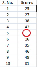
He made another blunder, he missed a couple of entries in a haste and we have no idea whose grades are lost. Let's find a way to solve this.

One way is that you visualize the grades and see if you can find a trend in the information.

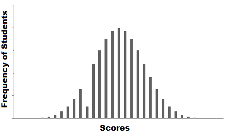
The graphical record that you rich person plot is called the frequency distribution of the data. You see that there is a smooth curve like structure that defines our data, but get along you notice an unusual person? We have an abnormally low pitch at a particular score range. So the best judge would be to take in missing values that remove the dent in the dispersion.

This is how you would hear to solve a veridical-life job using data analysis. For any Data Scientist, a student Oregon a practitioner, distribution is a must bed concept. IT provides the basis for analytics and connotative statistics.

While the conception of probability gives us the mathematical calculations, distributions help us actually visualize what's natural event underneath.

In this clause, I have covered some important probability distributions which are explained in a lucid as well as oecumenical fashion.

Note: This article assumes you take a basic knowledge of chance. If non, you can refer this chance distributions.

Common Data Types
Types of Distributions
1. Jean Bernoulli Dispersion
2. Uniform Distribution
3. Bernoulli distribution
4. Gaussian distribution
5. Poisson Distribution
6. Exponential Distribution
Relations between the Distributions
Test your Knowledge!

Popular Data Types

Before we get on to the explanation of distributions, let's see what kind of information backside we encounter. The data can be discrete Oregon continuous.

Discrete Data, atomic number 3 the name suggests, can take lone specified values. For instance, when you axial rotation a die, the possible outcomes are 1, 2, 3, 4, 5 or 6 and not 1.5 operating room 2.45.

Continuous Data can take any value within a given range. The range may be finite or infinite. E.g., A girl's exercising weight or height, the length of the road. The weight of a young woman can live any value from 54 kgs, or 54.5 kgs, Beaver State 54.5436kgs.

Today let us start with the types of distributions.

Types of Distributions

John Bernoull Dispersion

Lashkar-e-Tayyiba's start with the easiest dispersion that is Bernoulli Dispersion. It is actually easier to understand than IT sounds!

All you cricket junkies out there! At the beginning of whatever cricket twin, how do you decide who is exit to bat or formal? A toss! It every last depends on whether you profits or lose the toss, right? Rent out's say if the toss results in a head, you win. Else, you recede. On that point's no midway.

A Bernoulli distribution has only two contingent outcomes, namely 1 (success) and 0 (failure), and a single run. So the hit-or-miss variable X which has a Bernoulli distribution can take respect 1 with the probability of achiever, say p, and the value 0 with the probability of failure, say q or 1-p.

Here, the occurrence of a head denotes success, and the occurrence of a after part denotes unsuccessful person.
Probability of getting a head = 0.5 = Chance of acquiring a tail since there are only 2 possible outcomes.

The probability flock function is given by: p^x(1-p)^1-x where x € (0, 1).
It throne also be written atomic number 3

The probabilities of success and failure need not Be evenly likely, like the result of a scrap between me and Undertaker. He is bad much certain to profits. So in that case chance of my achiever is 0.15 while my failure is 0.85

Here, the probability of success(p) is not same atomic number 3 the chance of unsuccessful person. So, the chart below shows the Bernoulli distribution of our fight.

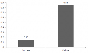
Here, the chance of success = 0.15 and chance of failure = 0.85. The expected value is exactly what IT sounds. If I punch you, I may expect you to punch Maine back. Essentially first moment of any statistical distribution is the mean of the distribution. The due value of a random variable X from a Bernoulli distribution is found as follows:

E(X) = 1*p + 0*(1-p) = p

The variance of a random variable from a John Bernoull distribution is:

V(X) = E(X²) – [E(X)]² = p – p² = p(1-p)

On that point are many an examples of Binomial distribution such as whether information technology's going away to pelting tomorrow or not where rain denotes success and no rainfall denotes failure and Winning (success) or losing (unsuccessful person) the game.

Uniform Dispersion

When you roll a impartial die, the outcomes are 1 to 6. The probabilities of getting these outcomes are equally likely and that is the basis of a uniform statistical distribution. Unlike Bernoulli Distribution, all the n number of possible outcomes of a uniform distribution are every bit promising.

A variable X is said to be uniformly divided up if the density purpose is:

The graph of a uniform distribution curve looks the likes of

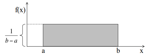
You rear end assure that the shape of the Unvarying distribution curve is rectangular, the reason why Uniform distribution is called rectangular distribution.

For a Uniform Distribution, a and b are the parameters.

The number of bouquets sold day-to-day at a flower shop is uniformly distributed with a maximum of 40 and a minimal of 10.

Let's try hard the probability that the daily sales bequeath fall between 15 and 30.

The chance that daily sales will fall between 15 and 30 is (30-15)*(1/(40-10)) = 0.5

Similarly, the probability that daily sales are greater than 20 is = 0.667

The mean and variance of X following a regular distribution is:

Mean -> E(X) = (a+b)/2

Variance -> V(X) = (b-a)²/12

The accepted uniform compactness has parameters a = 0 and b = 1, so the PDF for standard uniform density is given by:

Bernoulli distribution

Let's get rearwards to cricket. Suppose that you North Korean won the thrash about nowadays and this indicates a successful upshot. You toss again but you confounded this time. If you win a sky today, this does non necessitate that you will win the toss tomorrow. Let's impute a variant, say X, to the routine of times you won the toss. What can be the possible prise of X? It can be any number contingent the number of times you tossed a coin.

There are only 2 possible outcomes. Head denoting success and tail denoting failure. Therefore, probability of acquiring a head = 0.5 and the probability of failure can be well computed as: q = 1- p = 0.5.

A distribution where sole two outcomes are possible, such every bit achiever or bankruptcy, gain or red ink, win or lose and where the probability of success and unsuccessful person is same for all the trials is called a Binomial Distribution.

The outcomes need non glucinium equally likely. Remember the example of a combat between me and Mortician? So, if the chance of success in an experimentation is 0.2 then the probability of failure buttocks be easy computed as q = 1 – 0.2 = 0.8.

From each one trial is independent since the outcome of the previous toss doesn't determine or affect the outcome of the current toss. An try out with solitary two possible outcomes perennial n number of times is named language unit. The parameters of a binomial statistical distribution are n and p where n is the tote up numeral of trials and p is the probability of succeeder in each trial.

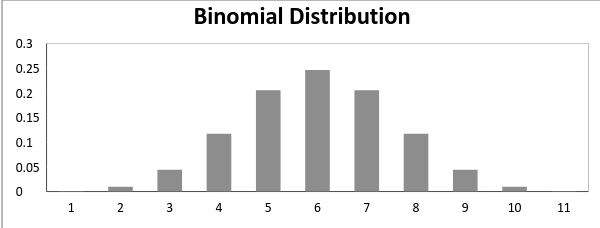
On the groundwork of the above explanation, the properties of a Binomial Dispersion are

Each test is independent.
In that location are only deuce possible outcomes in a trial- either a success or a failure.
A total number of n identical trials are conducted.
The probability of success and failure is same for all trials. (Trials are identical.)

The mathematical representation of Bernoulli distribution is given by:

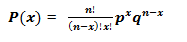
A Bernoulli distribution chart where the chance of succeeder does not isometrical the probability of failure looks like-minded

In real time, when probability of success = probability of failure, in such a situation the graph of Bernoulli distribution looks wish

The mean and variance of a linguistic unit distribution are apt away:

Mean -> µ = n*p

Variance -> Var(X) = n*p*q

Normal Distribution

Normal distribution represents the behavior of most of the situations in the universe (That is why it's named a "normal" distribution. I guess!). The large sum of (small) random variables often turns out to be normally distributed, contributing to its widespread application. Any distribution is called Normal distribution if it has the following characteristics:

The mean, median and way of the statistical distribution coincide.
The curve of the distribution is convex and rhombohedral about the line x=μ.
The total area under the bend is 1.
Exactly half of the values are to the left of the shopping centre and the other half to the right.

A median distribution is highly different from Binomial Statistical distribution. However, if the number of trials approaches infinity then the shapes will personify quite similar.

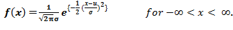
The PDF of a random variable X following a normal distribution is given by:

The think and variance of a random variable X which is said to be normally distributed is given past:

Imply -> E(X) = µ

Variance -> Var(X) = σ^2

Here, µ (stingy) and σ (standard deviation) are the parameters.
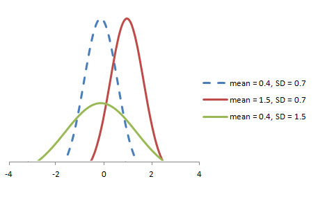
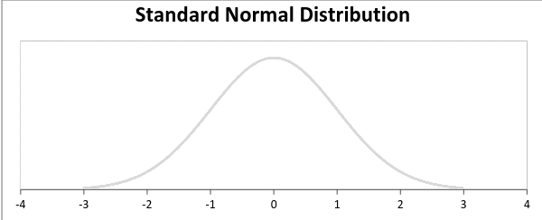
The graphical record of a variant X ~ N (µ, σ) is shown below.

A standard normal distribution is circumscribed American Samoa the dispersion with mean 0 and standard deviation 1. For such a display case, the PDF becomes:

Poisson Distribution

Suppose you work at a call center, approximately how umteen calls do you come in a day? It can be any enumerate. Now, the uncastrated number of calls at a call centre in a day is modeled by Poisson distribution. Roughly many examples are

The number of emergency brake calls recorded at a hospital in a day.
The number of thefts rumored in an domain happening a day.
The number of customers arriving at a salon in an hr.
The number of suicides reported in a particular city.
The number of printing errors at each page of the Good Book.

You can now think up many examples following the same course. Poisson Statistical distribution is applicable in situations where events occur indiscriminately points of time and space wherein our interest lies only in the number of occurrences of the case.

A distribution is called Poisson distribution when the following assumptions are valid:

1. Any successful consequence should non influence the outcome of some other booming event.
2. The probability of success all over a short interval must equal the probability of success over a longer separation.
3. The probability of success in an interval approaches zero as the time interval becomes smaller.

Now, if any distribution validates the above assumptions then information technology is a Poisson statistical distribution. Several notations used in Poisson distribution are:

λ is the rate at which an issue occurs,
t is the duration of a time interval,
And X is the number of events in that interval.

Present, X is called a Poisson Stochastic Variable and the probability distribution of X is titled Poisson distribution.

Army of the Pure µ denote the meanspirited number of events in an interval of length t. Then, µ = λ*t.

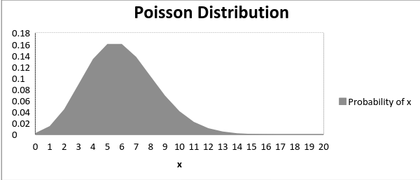
The PMF of X following a Poisson statistical distribution is given past:

The mean µ is the parameter of this distribution. µ is besides defined as the λ multiplication length of that interval. The graph of a Poisson distribution is shown below:

The graph shown below illustrates the shift in the trend due to increase in mean.

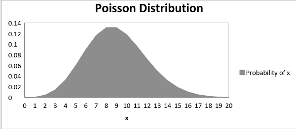
It is perceptible that as the mean increases, the curve ball shifts to the right.

The mean and variance of X following a Poisson distribution:

Mean -> E(X) = µ
Variance -> Var(X) = µ

Mathematical notation Statistical distribution

Let's consider the call centre example one more time. What about the separation of time between the calls ? Here, exponential distribution comes to our rescue. Exponential distribution models the interval of sentence between the calls.

Other examples are:

1. Length of time beteeen metro arrivals,
2. Length of clock time between arrivals at a gas station
3. The life of an Air Conditioner

Exponential dispersion is widely old for natural selection analysis. From the expected sprightliness of a machine to the expectable life of a human, exponential distribution successfully delivers the result.

A random versatile X is same to have an exponential distribution with PDF:

f(x) = { λe^-λx, x ≥ 0

and parameter λ>0 which is likewise called the rank.

For selection analysis, λ is named the failure rate of a device at any clock t, given that IT has survived capable t.

Mean and Variance of a unselected variable X following an exponential distribution:

Mean -> E(X) = 1/λ

Variance -> Volt-ampere(X) = (1/λ)²

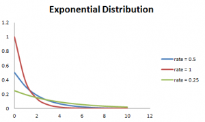
Also, the greater the rate, the quicker the arc drops and the lower the rate, flatter the curve. This is explained better with the graph shown on a lower floor.

To ease the computation, there are some formulas given below.
P{X≤x} = 1 – e^-λx, corresponds to the area under the density curve to the left of x.

P{X>x} = e^-λx, corresponds to the area under the density trend to the satisfactory of x.

P{x1<X≤ x2} = e^-λx1 – e^-λx2, corresponds to the area under the compactness curve between x1 and x2.

Relations between the Distributions

Intercourse 'tween Bernoulli and Binomial Distribution

1. Bernoulli Distribution is a special case of Binomial Dispersion with a one-person trial.

2. Thither are exclusively two possible outcomes of a Bernoulli and Quantity distribution, that is to say winner and unsuccessful person.

3. Both Bernoulli and Binomial Distributions have nonpartizan trails.

Sexual intercourse between Poisson and Binomial Dispersion

Poisson Statistical distribution is a restrictive case of binomial dispersion under the pursual conditions:

The number of trials is indefinitely mountainous operating theater n → ∞.
The chance of success for from each one trial is same and indefinitely undersized or p →0.
np = λ, is finite.

Relation between Normal and Bernoulli distribution &adenylic acid; Normal and Poisson distribution:

Gaussian distribution is another limiting form of Bernoulli distribution under the following conditions:

The number of trials is indefinitely capacious, n → ∞.
Both p and q are non indefinitely small.

The normal distribution is also a restricting case of Poisson distribution with the parameter λ →∞.

Relation 'tween Exponential and Poisson Distribution:

If the times 'tween random events pursue exponential distribution with rate λ, then the total number of events in a period of time of length t follows the Poisson distribution with parametric quantity λt.

Exam your knowledge

You have fall this far. Now, are you able to answer the following questions? Let me know in the comments below!

1. The formula to look classic normal random variable is:

a. (x+µ) / σ
b. (x-µ) / σ
c. (x-σ) / µ

2. In Jean Bernoulli Distribution, the formula for shrewd standard deflection is given by:

a. p (1 – p)
b. SQRT(p(p – 1))
c. SQRT(p(1 – p))

3. For a Gaussian distribution, an growth in the mean leave:

a. switch the curve to the left
b. shift the curve to the right
c. flatten the curve

4. The lifetime of a battery is exponentially distributed with λ = 0.05 per hour. The probability for A battery to last between 10 and 15 hours is:

a.0.1341
b.0.1540
c.0.0079

End Notes

Probability Distributions are prevalent in many sectors, namely, insurance, physics, engine room, electronic computer science and justified social science wherein the students of psychology and medical are widely exploitation probability distributions. It has an user-friendly application and distributed use. This clause highlighted six important distributions which are determined in day-to-solar day life and explained their applications programme. Now you will represent healthy to identify, relate and severalize among these distributions.

If you suffer any doubts and want to encounter more articles on distributions, please do spell in the comment section under. For a more in-depth indite dormie of these distributions, you fanny refer this resource.

I hope this article helps you in your data skill journey. Was it explanatory? Army of the Pure me screw in the comment section.

Learn, engage, compete, and get hired!